Structural material modeling tutorial
The scripts for generating data and running the tutorial sample problem can be found in the examples/structural-inference/tension directory in the full distribution package.
The tutorial solves a practical problem: given experimental tension test data for a material with varying material properties find a statistical viscoplastic model, defined by a set of model parameter distributions, that represents the resulting variation in the material response. The experimental data characterizes the variability in the material response. This variability may arise from heat-to-heat variation in the underlying material properties, caused by manufacturing variability, or from random experimental noise in the test controls and measurements.
There are three ingredients pyoptmat uses to generate a statistical model for the material behavior
Experimental data sampling different test conditions and the variability in the underlying material properties.
A parameterized mathematical model describing the material behavior. This model can be setup as as if it was deterministic, the inference process will find parameter distributions to explain the distribution of the test data.
Guesses as to what the statistical distribution of each model parameter should be. These are the formal prior parameter distributions for the statistical inference, and although they can be very poor guesses (“ill-informed priors”) the inference algorithm can still produce a very accurate statistical model.
Input data
The example works with synthetic experimental data. These data represent tension test results, given as stress/strain flow curves, at seven different strain rates: \(10^{-2}\) 1/s, \(10^{-3}\) 1/s, \(10^{-4}\) 1/s, \(10^{-5}\) 1/s, \(10^{-6}\) 1/s, \(10^{-7}\) 1/s, and \(10^{-8}\) 1/s. The material has some variability in the material properties that determine the experimental measurements. So each repetition of a test at a particular strain rate will produce a somewhat different flow curve. To capture this variability the test data includes 50 repeated tests at each strain rate, for 350 tests data. However, far fewer repeated tests are actually needed to produce a good statistical model of the material behavior.

Plot showing the variation in the tensile flow curves for a strain rate of \(10^{-2}\) 1/s for a parameter scale of 0.05.
For this example the data is “synthetic.” That is, it is not actual tests data but rather data generated through the material model, described below, using known parameter distributions. The goal here is to validate the methods used by pyoptmat by recovering these known property distributions through statistical inference over the synthetic data.
To test the reliability of pyoptmat for different amounts of material variability, the provided data includes five datasets, each with a different level of material property variability. The example generates the synthetic data by simulating experiments using the model where all the model parameters, except the Young’s modulus, are sampled from normal distributions with the parameters scaled so that the mean of each distribution is 0.5. The five datasets are then from distributions with increasing variability, specifically the parameter distributions have standard deviations of 0.0, 0.01, 0.05, 0.1, and 0.15. Increasing variability in the parameter distributions translates to increased scatter in the synthetic tension test data, representing, for example, materials with larger heat-to-heat variations caused by looser manufacturing process controls.
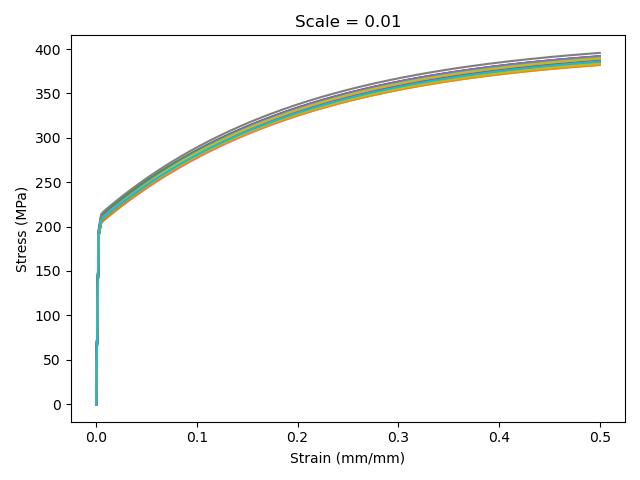
Plot showing the variation in the tensile flow curves for a strain rate of \(10^{-2}\) 1/s for a parameter scale of 0.01…
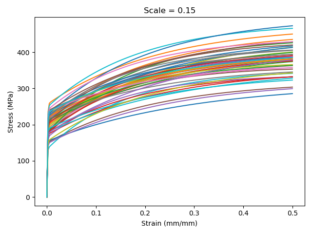
… compared the variation at the same strain rate for a scale of 0.15.
pyoptmat has the ability to infer the level of random noise in the experimental data, separate from the statistical variation in the material properties caused by heat-to-heat variation. However, this synthetic dataset does not include any noise, i.e. all the variation in the response is caused by the distribution of the material properties.
The example directory contains pregenerated datasets for the aforementioned five levels of material variability. Therefore, in following this example you do not need to generate the synthetic test data. However, running the examples/structural-inference/tension/maker.py script (below) will regenerate the test data, by simulating tension tests with model parameters sampled from the assumed parameter distributions.
Mathematical model
This example uses a viscoplastic constitutive model with isotropic hardening to describe the material behavior. Mathematically, this model is a system of two ordinary differential equations driving by the input strain and time data from the experiments. The first ODE in the system describes the evolution of stress with time:
with
In these expressions \(\dot{\varepsilon}\) is the strain rate driving material deformation, \(E\) iss the material Youngs modulus, \(\sigma\) is the current stress, \(\sigma_0\) is a threshold stress, \(\eta\) is the flow fluidity, \(n\) is the rate sensitivity, and \(K\) is the isotropic hardening, defined below. The initial condition for this ODE is zero, i.e. the material starts in an unloaded state.
The second ODE describes the evolution of the isotropic hardening
where \(R\) is the saturated isotropic hardening strength, \(\delta\) describes how fast the hardening saturates, and the initial condition is again zero.
This model has 6 parameters: - \(E\) the Young’s modulus - \(n\) the rate sensitivity - \(\eta\) the flow fluidity - \(\sigma_0\) the threshold stress - \(\delta\) the isotropic hardening saturation parameter - \(R\) the saturated isotropic hardening
The model is parameterized so that the synthetic experimental data is generated with distributions where all these parameter values are 0.5. That is, 0.5 is the true mean of the parameter distribution for all the parameters. In actual materials there is comparatively little heat-to-heat variation in the material Young’s modulus \(E\). Therefore, the analysis here treats the Young’s modulus as deterministic and fixed to a value of 0.5, both in generating the synthetic data and in developing the statistical model.
This leaves five parameters. The goal of the statistical inference is to find distributions of these five parameters that explain the variation in the experimental data.
pyoptmat can infer the amount of random noise in the test data, in addition to inferring property distributions explaining the heat-to-heat variation in the underlying material properties. Models in pyopmat account for these random variations through Gaussian noise additively superimposed with the simulated distribution of stress from the stochastic ODEs.
In this example the data does not have any noise and so the model does not infer the scale of this white noise term. Instead the analysis fixes the scale of the noise to a very small value (\(10^{-4}\)), which is essentially zero.
Statistical inference
The script examples/structural-inference/tension/statistics/infer.py (listed below) sets up the model and performs statistical variational inference to find the model parameter distributions. The script imports two utility functions from examples/structural-inference/tension/maker.py also used in generating the synthetic data. The following walks through infer.py and those two functions to explain how to load in experimental data, setup a statistical model, provide prior distributions, and run the interference.
Setup
The inference script relies on several other modules in pyoptmat, pyro, numpy, matplotlib, and xarray:
#!/usr/bin/env python3

import sys
import os.path
sys.path.append('../../../..')
sys.path.append('..')

import numpy as np
import numpy.random as ra

import xarray as xr
import torch

from maker import make_model, downsample

from pyoptmat import optimize, experiments
from tqdm import tqdm

import pyro
from pyro.infer import SVI, Trace_ELBO
import pyro.optim as optim

import matplotlib.pyplot as plt
During inference, the parameter distributions might sample invalid or difficult parts of the parameter space where integrating the model becomes difficult. Usually this does not affect the final results and so the script suppresses the warnings pyoptmat provides when integration fails:
import warnings
warnings.filterwarnings("ignore")
Accurately integrating models of this type requires using double precision arithmetic.
# Use doubles
torch.set_default_tensor_type(torch.DoubleTensor)
The next block of code sets up the problem to run on the GPU using CUDA, if available, or falls back on the CPU if CUDA is not available. torch will use OpenMP to run in parallel in multiple cores on the CPU. This behavior may not be desirable, depending on your system setup, and can be suppressed by setting OMP_NUM_THREADS=1 in the system, for example as an environment variable at the command line.
# Run on GPU!
if torch.cuda.is_available():
    dev = "cuda:0"
else:
    dev = "cpu"
device = torch.device(dev)
The model maker function
This is all the setup code. The example relies on a “maker” function. This function takes the model parameters as input and returns the initialize pyoptmat model. pyoptmat relies on these “maker” functions to abstract the type of model – deterministic or statistical. Armed with this maker function the package can either initialize the parameters as pytorch Parameters or pyro samples and reuse the same code for both deterministic and statistical models.
The example uses two functions to define the final maker. The first function is in maker.py
def make_model(E, n, eta, s0, R, d, device = torch.device("cpu"), **kwargs):
  """
    Key function for the entire problem: given parameters generate the model
  """
  isotropic = hardening.VoceIsotropicHardeningModel(
      CP(R, scaling = optimize.bounded_scale_function((torch.tensor(R_true*(1-sf), device = device), torch.tensor(R_true*(1+sf), device = device)))),
      CP(d, scaling = optimize.bounded_scale_function((torch.tensor(d_true*(1-sf), device = device), torch.tensor(d_true*(1+sf), device = device)))))
  kinematic = hardening.NoKinematicHardeningModel()
  flowrule = flowrules.IsoKinViscoplasticity(
      CP(n, scaling = optimize.bounded_scale_function((torch.tensor(n_true*(1-sf), device = device), torch.tensor(n_true*(1+sf), device = device)))),
      CP(eta, scaling = optimize.bounded_scale_function((torch.tensor(eta_true*(1-sf), device = device), torch.tensor(eta_true*(1+sf), device = device)))),
      CP(s0, scaling = optimize.bounded_scale_function((torch.tensor(s0_true*(1-sf), device = device), torch.tensor(s0_true*(1+sf), device = device)))),
      isotropic, kinematic)
  model = models.InelasticModel(CP(E, scaling = optimize.bounded_scale_function((torch.tensor(E_true*(1-sf), device = device), torch.tensor(E_true*(1+sf), device = device)))),
      flowrule)

  return models.ModelIntegrator(model, **kwargs)
This function constructs a fully-parameterized instantiation of the model, including the Young’s modulus \(E\). The kwargs are used to place the model on the appropriate device (CPU and GPU) and any additional arguments are passed to the model integrator. This function mirrors the mathematical description above exactly.
Note that the CP object is the pyoptmat.temperature.ConstantParameter class imported from the
pyoptmat.temperature modules. It means that the model parameters in this example do not depend on
temperature.
The infer.py script wraps this maker function with a small additional function:
# Don't try to optimize for the Young's modulus
def make(n, eta, s0, R, d, **kwargs):
  return make_model(torch.tensor(0.5), n, eta, s0, R, d,
      device = device, **kwargs).to(device)
which enforces the condition described above, that the Young’s modulus is deterministic, fixed to the correct value (0.5), and not included in the statistic inference.
With the maker function defined the main script loads “experimental” data, sets up prior distributions for the parameters, and completes the inference for the parameter distributions.
Loading data
The example problem loads 10 of the 50 repeated trials from the case with the known parameter scale of 0.05:
# 1) Load the data for the variance of interest,
#    cut down to some number of samples, and flatten
scale = 0.05
nsamples = 10 # at each strain rate
input_data = xr.open_dataset(os.path.join('..', "scale-%3.2f.nc" % scale))
data, results, cycles, types, control = downsample(experiments.load_results(
    input_data, device = device),
    nsamples, input_data.nrates, input_data.nsamples)
By default the pyoptmat.experiments.load_results() function loads all of the experimental data in the
xarray file. The downsample function is defined in maker.py and reduces the dataset from the 50 full repeats at each
strain rate down to the number requested, here 10.
def downsample(rawdata, nkeep, nrates, nsamples):
  """
    Return fewer than the whole number of samples for each strain rate
  """
  ntime = rawdata[0].shape[1]
  return tuple(data.reshape(data.shape[:-1] + (nrates, nsamples))[...,:nkeep].reshape(data.shape[:-1]+(-1,))
      for data in rawdata)
Prior distributions
The next step is to provide some human readable names for the model parameters and then define the parameter prior distributions.
# 2) Setup names for each parameter and the priors
names = ["n", "eta", "s0", "R", "d"]
loc_loc_priors = [torch.tensor(ra.random(), device = device) for i in range(len(names))]
loc_scale_priors = [torch.tensor(0.15, device = device) for i in range(len(names))]
scale_scale_priors = [torch.tensor(0.15, device = device) for i in range(len(names))]

eps = torch.tensor(1.0e-4, device = device)

print("Initial parameter values:")
print("\tloc loc\t\tloc scale\tscale scale")
for n, llp, lsp, sp in zip(names, loc_loc_priors, loc_scale_priors,
    scale_scale_priors):
  print("%s:\t%3.2f\t\t%3.2f\t\t%3.2f" % (n, llp, lsp, sp))
print("")
The names array is just an array of string names, one for each parameter in the order they
are passed to the maker function. The next three lists define the prior distributions, one
for each parameter. The statistical model put together here is a
pyoptmat.optimize.HierarchicalStatisticalModel with two levels of statistical
distributions. At the bottom level the model first samples from random variables representing the
heat-specific model properties. In the current implementation these distributions are
taken as normal distributions, meaning they are defined by a location parameter, giving the mean,
and a scale parameter, giving the standard deviation.
This example assumes each test is drawn from a random heat (or, equivalently, each sample is from
a separate heat) and so once the model determines lower-level normal distribution for each parameter
it then samples those distributions once for each test, independently.
In the hierarchical model the heat-specific mean and standard deviation are themselves random variables. The mean of the heat-specific distributions is given itself by a normal distribution, again described by the location and scale parameter. The scale of the heat-specific distributions are given by half normal distributions, parameterized by a scale parameter.
So three values define the statistical model for each parameter: the location and scale of the normal distribution
describing the heat-specific mean and the scale parameter defining the scale of the heat-specific mean.
The prior distributions can then be defined with initial guesses for each of these three parameters.
The loc_loc_priors, code_scale_priors, and scale_scale_priors define these priors for each
model parameter. In this example the locations (i.e. mean parameter values) are selected random from the range
[0,1] (again recall the true mean parameter values used to generate the data are 0.5). The scale parameters are all
set to 0.15 (recall the true scale in this example is 0.05).
These choices are generally good for models using real material data: the prior describing the location of each parameter distribution can be ill-informed and the scale of the priors should be set so that they produce greater variance than in the actual test data.
The parameters in this example are scaled not only for convenience but for numerical reasons. The “natural” model parameters for the material model should be scaled so that they all have values of around 1.0.
As noted above, while pyopmat can infer the level of noise in the experimental data, this example does not include any random error caused by experimental variability and so the scale of the white noise is fixed to a small value (\(10^{-4}\)).
Finally, the model prints out information on the prior values. The location priors will vary, as they are random, but the output will look something like this:
Initial parameter values:
     loc loc         loc scale       scale scale
n:   0.37            0.15            0.15
eta: 0.52            0.15            0.15
s0:  0.75            0.15            0.15
R:   0.35            0.15            0.15
d:   0.48            0.15            0.15
Setting up the model and optimizer
The next steps are to setup the
pyoptmat.optimize.HierarchicalStatisticalModel object,
initialize the guide distribution, and setup the optimizer used to
solve the problem.
# 3) Create the actual model
model = optimize.HierarchicalStatisticalModel(make, names, loc_loc_priors,
    loc_scale_priors, scale_scale_priors, eps).to(device)

# 4) Get the guide
guide = model.make_guide()

# 5) Setup the optimizer and loss
lr = 1.0e-2
g = 1.0
niter = 200
lrd = g**(1.0 / niter)
num_samples = 1

optimizer = optim.ClippedAdam({"lr": lr, 'lrd': lrd})
We generally suggest using a ClippedAdam optimizer. The learning rate in
this example is too high for real experimental data. We have found
learning rates around \(10^{-3}\) work well for actual data.
The hyperparameters here configure geometric learning rate decay with
rate g. However, for this simple example this heuristic is not required
to produce good results. For real data we have found \(g=0.9\) or so
can help with convergence.
Statistical Variation Inference and running the problem
We can now set up the pyro ELBO objective function and the SVI problem and solve the inference problem.
ls = pyro.infer.Trace_ELBO(num_particles = num_samples)

svi = SVI(model, guide, optimizer, loss = ls)

# 6) Infer!
t = tqdm(range(niter), total = niter, desc = "Loss:    ")
loss_hist = []
for i in t:
  loss = svi.step(data, cycles, types, control, results)
  loss_hist.append(loss)
  t.set_description("Loss %3.2e" % loss)
There num_samples is the number of samples to use in calculating the
ELBO values. We have not found increasing this from 1 to help with convergence.
The example will print a progress bar while it is determining the inferred distributions
Loss 3.02e+11: 42%|███████████▍ | 85/200 [11:40<15:52, 8.29s/it]
Results
The script will print the inferred posterior distributions and plot the convergence history
# 7) Print out results
print("")
print("Inferred distributions:")
print("\tloc\t\tscale")
for n in names:
  s = pyro.param(n + model.scale_suffix + model.param_suffix).data
  m = pyro.param(n + model.loc_suffix + model.param_suffix).data
  print("%s:\t%3.2f/0.50\t%3.2f/%3.2f" % (n,
    m,
    s,
    scale))
print("")

# 8) Plot convergence
plt.figure()
plt.loglog(loss_hist)
plt.xlabel("Iteration")
plt.ylabel("Loss")
plt.tight_layout()
plt.show()
The convergence history for this example is less smooth than for a better, smaller learning rate

Convergence history for one run of the sample problem. A smaller learning rate and more iterations would produce better convergence and, potentially, a more accurate model.
However, the final results are reasonable:
Inferred distributions:
      loc            scale
n:   0.50/0.50       0.02/0.05
eta: 0.49/0.50       0.02/0.05
s0:  0.49/0.50       0.03/0.05
R:   0.48/0.50       0.05/0.05
d:   0.48/0.50       0.05/0.05
Because the priors are randomized your results will vary. However, these results are fairy typical, even for real data. pyoptmat usually does a very good job establishing the mean of the parameter distributions – the results here are very close to the true mean of 0.5 – and typically somewhat underestimates the true variance, which is a problem common to most variational Bayes approaches.
Despite somewhat underestimating the true variance the model still does a very good job in capturing the actual variation in the synthetic test data.
maker.py: script for regenerating the synthetic test data
#!/usr/bin/env python3

"""
    Helper functions for the structural material model inference with
    tension tests examples.
"""

import sys

sys.path.append("../../..")

import numpy as np
import numpy.random as ra

import xarray as xr

import torch
from pyoptmat import models, flowrules, hardening, optimize
from pyoptmat.temperature import ConstantParameter as CP

from tqdm import tqdm

import tqdm

import warnings

warnings.filterwarnings("ignore")

# Use doubles
torch.set_default_tensor_type(torch.DoubleTensor)

# Actual parameters
E_true = 150000.0
R_true = 200.0
d_true = 5.0
n_true = 7.0
eta_true = 300.0
s0_true = 50.0

# Scale factor used in the model definition
sf = 0.5

# Select device to run on
if torch.cuda.is_available():
    dev = "cuda:0"
else:
    dev = "cpu"
device = torch.device(dev)


def make_model(E, n, eta, s0, R, d, device=torch.device("cpu"), **kwargs):
    """
    Key function for the entire problem: given parameters generate the model
    """
    isotropic = hardening.VoceIsotropicHardeningModel(
        CP(
            R,
            scaling=optimize.bounded_scale_function(
                (
                    torch.tensor(R_true * (1 - sf), device=device),
                    torch.tensor(R_true * (1 + sf), device=device),
                )
            ),
        ),
        CP(
            d,
            scaling=optimize.bounded_scale_function(
                (
                    torch.tensor(d_true * (1 - sf), device=device),
                    torch.tensor(d_true * (1 + sf), device=device),
                )
            ),
        ),
    )
    kinematic = hardening.NoKinematicHardeningModel()
    flowrule = flowrules.IsoKinViscoplasticity(
        CP(
            n,
            scaling=optimize.bounded_scale_function(
                (
                    torch.tensor(n_true * (1 - sf), device=device),
                    torch.tensor(n_true * (1 + sf), device=device),
                )
            ),
        ),
        CP(
            eta,
            scaling=optimize.bounded_scale_function(
                (
                    torch.tensor(eta_true * (1 - sf), device=device),
                    torch.tensor(eta_true * (1 + sf), device=device),
                )
            ),
        ),
        CP(
            s0,
            scaling=optimize.bounded_scale_function(
                (
                    torch.tensor(s0_true * (1 - sf), device=device),
                    torch.tensor(s0_true * (1 + sf), device=device),
                )
            ),
        ),
        isotropic,
        kinematic,
    )
    model = models.InelasticModel(
        CP(
            E,
            scaling=optimize.bounded_scale_function(
                (
                    torch.tensor(E_true * (1 - sf), device=device),
                    torch.tensor(E_true * (1 + sf), device=device),
                )
            ),
        ),
        flowrule,
    )

    return models.ModelIntegrator(model, **kwargs)


def generate_input(erates, emax, ntime):
    """
    Generate the times and strains given the strain rates, maximum strain, and number of time steps
    """
    strain = torch.repeat_interleave(
        torch.linspace(0, emax, ntime, device=device)[None, :], len(erates), 0
    ).T.to(device)
    time = strain / erates

    return time, strain


def downsample(rawdata, nkeep, nrates, nsamples):
    """
    Return fewer than the whole number of samples for each strain rate
    """
    ntime = rawdata[0].shape[1]
    return tuple(
        data.reshape(data.shape[:-1] + (nrates, nsamples))[..., :nkeep].reshape(
            data.shape[:-1] + (-1,)
        )
        for data in rawdata
    )


if __name__ == "__main__":
    # Running this script will regenerate the data
    ntime = 200
    emax = 0.5
    erates = torch.logspace(-2, -8, 7, device=device)
    nrates = len(erates)
    nsamples = 50

    scales = [0.0, 0.01, 0.05, 0.1, 0.15]

    times, strains = generate_input(erates, emax, ntime)

    for scale in scales:
        print("Generating data for scale = %3.2f" % scale)
        full_times = torch.empty((ntime, nrates, nsamples), device=device)
        full_strains = torch.empty_like(full_times)
        full_stresses = torch.empty_like(full_times)
        full_temperatures = torch.zeros_like(full_strains)

        for i in tqdm.tqdm(range(nsamples)):
            full_times[:, :, i] = times
            full_strains[:, :, i] = strains

            # True values are 0.5 with our scaling so this is easy
            model = make_model(
                torch.tensor(0.5, device=device),
                torch.tensor(ra.normal(0.5, scale), device=device),
                torch.tensor(ra.normal(0.5, scale), device=device),
                torch.tensor(ra.normal(0.5, scale), device=device),
                torch.tensor(ra.normal(0.5, scale), device=device),
                torch.tensor(ra.normal(0.5, scale), device=device),
            )

            with torch.no_grad():
                full_stresses[:, :, i] = model.solve_strain(
                    times, strains, full_temperatures[:, :, i]
                )[:, :, 0]

        full_cycles = torch.zeros_like(full_times, dtype=int, device=device)
        types = np.array(["tensile"] * (nsamples * len(erates)))
        controls = np.array(["strain"] * (nsamples * len(erates)))

        ds = xr.Dataset(
            {
                "time": (["ntime", "nexp"], full_times.flatten(-2, -1).cpu().numpy()),
                "strain": (
                    ["ntime", "nexp"],
                    full_strains.flatten(-2, -1).cpu().numpy(),
                ),
                "stress": (
                    ["ntime", "nexp"],
                    full_stresses.flatten(-2, -1).cpu().numpy(),
                ),
                "temperature": (
                    ["ntime", "nexp"],
                    full_temperatures.cpu().flatten(-2, -1).numpy(),
                ),
                "cycle": (["ntime", "nexp"], full_cycles.flatten(-2, -1).cpu().numpy()),
                "type": (["nexp"], types),
                "control": (["nexp"], controls),
            },
            attrs={"scale": scale, "nrates": nrates, "nsamples": nsamples},
        )

        ds.to_netcdf("scale-%3.2f.nc" % scale)
infer.py: inferring the model parameter distributions
#!/usr/bin/env python3

"""
    Tutorial example of training a statistical model to tension test data
    from from a known distribution.
"""

import sys
import os.path

sys.path.append("../../../..")
sys.path.append("..")

import numpy.random as ra

import xarray as xr
import torch

from maker import make_model, downsample

from pyoptmat import optimize, experiments
from tqdm import tqdm

import pyro
from pyro.infer import SVI
import pyro.optim as optim

import matplotlib.pyplot as plt

import warnings

warnings.filterwarnings("ignore")

# Use doubles
torch.set_default_tensor_type(torch.DoubleTensor)

# Run on GPU!
if torch.cuda.is_available():
    dev = "cuda:0"
else:
    dev = "cpu"
device = torch.device(dev)

# Don't try to optimize for the Young's modulus
def make(n, eta, s0, R, d, **kwargs):
    """
        Maker with Young's modulus fixed
    """
    return make_model(torch.tensor(0.5), n, eta, s0, R, d, device=device, **kwargs).to(
        device
    )


if __name__ == "__main__":
    # Number of vectorized time steps
    time_chunk_size = 40
    # Method to use to solve linearized implicit systems
    linear_solve_method = "pcr"

    # 1) Load the data for the variance of interest,
    #    cut down to some number of samples, and flatten
    scale = 0.05
    nsamples = 10  # at each strain rate
    input_data = xr.open_dataset(os.path.join("..", "scale-%3.2f.nc" % scale))
    data, results, cycles, types, control = downsample(
        experiments.load_results(input_data, device=device),
        nsamples,
        input_data.nrates,
        input_data.nsamples,
    )

    # 2) Setup names for each parameter and the priors
    names = ["n", "eta", "s0", "R", "d"]
    loc_loc_priors = [
        torch.tensor(ra.random(), device=device) for i in range(len(names))
    ]
    loc_scale_priors = [torch.tensor(0.15, device=device) for i in range(len(names))]
    scale_scale_priors = [torch.tensor(0.15, device=device) for i in range(len(names))]

    eps = torch.tensor(1.0e-4, device=device)

    print("Initial parameter values:")
    print("\tloc loc\t\tloc scale\tscale scale")
    for n, llp, lsp, sp in zip(
        names, loc_loc_priors, loc_scale_priors, scale_scale_priors
    ):
        print("%s:\t%3.2f\t\t%3.2f\t\t%3.2f" % (n, llp, lsp, sp))
    print("")

    # 3) Create the actual model
    model = optimize.HierarchicalStatisticalModel(
            lambda *args, **kwargs: make(*args, block_size = time_chunk_size, direct_solve_method = linear_solve_method,
                **kwargs),
            names, loc_loc_priors, loc_scale_priors, scale_scale_priors, eps
    ).to(device)

    # 4) Get the guide
    guide = model.make_guide()

    # 5) Setup the optimizer and loss
    lr = 1.0e-2
    g = 1.0
    niter = 200
    lrd = g ** (1.0 / niter)
    num_samples = 1

    optimizer = optim.ClippedAdam({"lr": lr, "lrd": lrd})

    ls = pyro.infer.Trace_ELBO(num_particles=num_samples)

    svi = SVI(model, guide, optimizer, loss=ls)

    # 6) Infer!
    t = tqdm(range(niter), total=niter, desc="Loss:    ")
    loss_hist = []
    for i in t:
        loss = svi.step(data, cycles, types, control, results)
        loss_hist.append(loss)
        t.set_description("Loss %3.2e" % loss)

    # 7) Print out results
    print("")
    print("Inferred distributions:")
    print("\tloc\t\tscale")
    for n in names:
        s = pyro.param(n + model.scale_suffix + model.param_suffix).data
        m = pyro.param(n + model.loc_suffix + model.param_suffix).data
        print("%s:\t%3.2f/0.50\t%3.2f/%3.2f" % (n, m, s, scale))
    print("")

    # 8) Plot convergence
    plt.figure()
    plt.loglog(loss_hist)
    plt.xlabel("Iteration")
    plt.ylabel("Loss")
    plt.tight_layout()
    plt.show()